In the past year, QAequilibraE development has been at full speed. There are too many improvements to list, including substantial work on the installation process, but we can highlight the following as the most important features:

• Route Choice
• Transit Assignment
• Select Link Analysis
• Tool access via Processing Provider

The latest significant improvement was recently made available in QAequilibraE’s release v1.4.4, but we didn’t talk much about it so far.

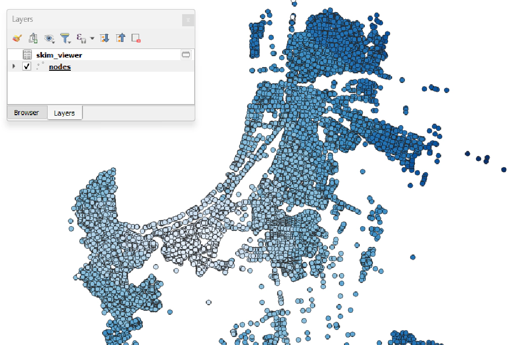
The tool we have dubbed Skim Viewer, is targeted at improving the quality (and speed) of data analysis for QGIS users, and it consists of allowing the user to easily and dynamically visualise network costs at each node or traffic analysis zone (TAZ) for paths starting at any node in the network.

QAequilibraE users might already know the mapping tool for matrix data, which allows users to map rows or columns of a skim matrix in an interactive way, which was a great feature to add. With Skim Viewer, users can go a step further in the analysis, uncover differences within zones, and visualise costs for metrics that they might not have skimmed.

To use Skim Viewer, the user doesn’t need skim matrices at all. Unlike the visualisation of matrix data, it’s not restricted to the TAZs, allowing the user to choose between network nodes and TAZs, which are computed and displayed on the fly.

Another particularity of Skim Viewer is that it allows the user to plot network costs based on any data available on the link layer (natively or through a join). Suppose you just ran a traffic assignment and want to check the congested time skims, tolls or some other measure of generalised cost. After configuring the graph with the field it should use to compute paths and the field to display, Skim Viewer recalculates and displays the new costs every time the user clicks in the map canvas, selecting the closest node as the new origin. When changing the graph configurations, such as minimising and skimming fields, the entire graph is automatically recomputed, and the new costs are plotted.

This makes for an incredibly dynamic visualisation of path costs through the network, and an easy way to inspect the model before and after traffic assignment.

About the implementation

The algorithmic implementation for Skim Viewer leverages AequilibraE’s path computation API, which allows the user to compute the shortest path tree between the desired start node/zone and all other nodes/zones in the model almost instantly. This is different from what is done in skimming (all-to-all), allowing Skim Viewer to quickly recompute the desired network costs when changing the initial node and plotting it. The computation is so fast that almost all the time taken to refresh the map is due to QGIS map rendering.

Get started with Skim Viewer today: Update to QAequilibraE v25.202.21 and look for the skim viewer option in the Paths and Assignment menu. Not sure where to begin? Check out our step-by-step tutorial.

Have a specific use case in mind? We’d love to feature it in a future blog post!

See you all in the next release!