Instant Project Dashboards for AequilibraE
Over the last two months, I have been interning with Outer Loop on the integration of web-based visualization …


Over the past 8 weeks we – Evelyn Bond and Tyler Pearn – have been working with Outer Loop as part of the University of Queensland SMP internship program. Our focus has been on taking prototype Mixed Logit Model estimation software developed by Outer Loop’s Principal Scientist Dr. Jan Zill, and packaging it into a modern, professional Python package that follows best practices, suitable for use by the wider Python and choice modelling communities.
The package we developed is called jaxlogit and is derived from the existing xlogit package. jaxlogit extends xlogit by leveraging JAX, a Just-in-Time (JIT) compiled high-performance numerical computing and ML library from Google. This allows for automatic differentiation of gradients of correlated random variables, increased performance, and ability to handle larger problem sizes.
We are very happy to announce that jaxlogit is now publicly available on PyPI as a stable 1.0 version and can be installed using pip:
pip install jaxlogit
During our work, we’ve taken inspiration from other modern professional packages in the Python ecosystem, such as Pandas and SciPy, and have identified a number of CI automations used by these packages and that we want to emulate:
Python packages are increasingly turning to automated tools such as ruff to automate and enforce the use of a standardised style guide. By adopting these standards early in the development and automating their enforcement in our CI pipelines, we entirely avoid any debates about the “correct” number of spaces to use for indenting or how long is too long for a line length. Automated linting can also flag issues such as misspelled variables names or type incompatibilities which would otherwise only be found at runtime in an interpreted language such as Python.
Unit tests were a priority for this project to provide a safety net for refactoring. To be useful, unit tests need to be fast and test all parts of the software systematically. We ran these using GitHub CI to ensure commits are always functioning. To this, we added branch coverage metrics and configured GitHub to generate reports on each commit. This allowed us to ensure our tests were targeted rather than relying on a coverage target. We measured branch coverage to check that the different options in the package were tested.
We also created tests for the whole system using real datasets. These caught a few bugs!
jaxlogit’s documentation is made using Sphinx, run through GitHub CI, and deployed using GitHub pages on pull request. This means the theming and structure is consistent with other open-source packages and ensures it is up to date and attached to the repository. We have also added an API reference generated from the code and included clear usage examples so that modellers can see it used on real problems and get started quickly.
The documentation can be found here.
Additionally, we wanted to reduce the learning curve for new users as much as possible and have implemented a wrapper around jaxlogit which allows it to be directly plugged into Scikit-Learn’s interface. This allows the use of Scikit-Learn’s existing tools like cross validation and grid search and makes jaxlogit plug-in compatible with existing estimation practices.
All the automated testing in the world isn’t helpful if the core goal of the package – accurate estimation of mixed logit models – isn’t achieved. Thankfully, there are a number of existing estimation packages available, including our direct ancestor xlogit, which provide us with robust reference data.
To ensure jaxlogit is accurate and useful, we compared its results and speed with xlogit and Biogeme, a general estimation package. To compare results, we will focus on the log likelihood of the found coefficients (the objective function that is maximised) and the model’s Brier score. The model’s Brier score measures how close the alternatives chosen by the agents are to our predicted probabilities from 0 (all correct) to 1 (all wrong). The table below shows these for the electricity dataset. This was calculated with an 80-20 train-test split.
| jaxlogit | xlogit | Biogeme | |
|---|---|---|---|
| Log Likelihood | 886.102 | 886.094 | 884.2682 |
| Brier Score | 0.624247 | 0.624247 | 0.624163 |
As evidenced by the identical Brier scores (to 3 decimal places) for jaxlogit and xlogit, the overall performance of the resulting models is identical. These results provide confidence that the models produced by jaxlogit are suitable as drop-in replacements for those estimated by xlogit and Biogeme.
We also created full system tests that perform estimation on the electricity dataset, and other popular discrete choice datasets such as the Swissmetro dataset . These can be found at the documentation for jaxlogit here.
To demonstrate the relative performance of the jaxlogit package, we repurposed and extended the benchmarking notebooks found in xlogit here. We looked at both runtime and memory usage when estimating a mixed logit model using both the artificial datasets and the more challenging dataset provided by Ken Train and David Revelt for electricity provider choice.
When running large model estimation tasks, often memory usage becomes a limiting factor. One way that this can be alleviated is using batching to break the problem into smaller sub-problems, each of which can be solved independently. This is a new feature that was added in jaxlogit and isn’t available in xlogit or Biogeme.
In the following plot we show the memory usage of the three packages as they solve the electricity datasetet. As can be seen in the graph below, the use of batching reduces the jaxlogit peak memory usage by approximately 60% allowing for solutions to be generated on systems with considerably less installed memory. Biogeme was removed because its peak was over 30GB and it distorted the graph.
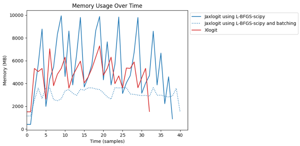
This reduction in memory usage isn’t completely free however, as there is computational overhead in the splitting and merging of the sub-problems. The overall increase in runtime when enabling batching can vary between 5-20% depending on the size of the problem and batch size used.
An additional insight that we took from this analysis was the jagged saw-tooth shape of the memory usage in jaxlogit. We dug into this further and found that there was significant overhead from data being constantly passed between JAX (which handles the calculation of the objective function and gradient) and the SciPy optimization routines (which handle the actual L-BFGS search). This motivated us to integrate a pure JAX optimizer (from Google) which allowed us to avoid these data transfers and leverage JIT across more of the computation for significantly faster overall runtimes.
The JAX-based optimiser performs significantly faster but exhibits higher peak memory usage. In our earlier testing, the peak memory usage of the JAX optimiser was about 20% higher at 12GB than at 10GB when using the SciPy optimiser. Unfortunately, the batching operation is currently only compatible with the SciPy-based optimiser.
One of the motivating factors for this work was the ability to use more draws in estimation. For Mixed logit models, we assume the coefficients of the explanatory variables, for example, the travel time and cost of each alternative, are randomly distributed according to unknown parameters. During estimation, we need to integrate over this distribution, which can only be done numerically. By drawing more often from this distribution, we more closely approximate the integral and decrease the variance of the solution.
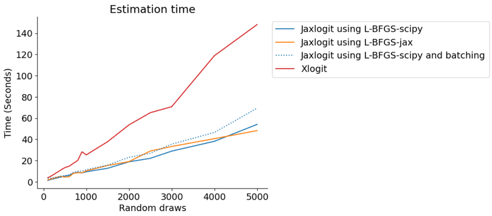
To demonstrate the ability of jaxlogit to handle more draws, we expanded the artificial dataset analysis above from a maximum of 300 draws as used by the xlogit notebooks to over 5000. The relative runtime for the various packages is shown in the below chart. Note that Biogeme isn’t included on this graph due to technical difficulties running it locally but xlogit’s testing shows that Biogeme performs significantly slower than xlogit.
L-BFGS-scipy refers to using the L-BFGS-B method with the default jaxlogit optimiser and L-BFGS-jax refers to using the L-BFGS method with Google’s jax optimiser. From this we can see that runtimes for both xlogit and jaxlogit are fairly linear with respect to the number of draws, but jaxlogit is twice as fast as xlogit (for all optimisation methods including batching). Interestingly, all optimisation methods of jaxlogit perform similarly – we believe this is likely because of the small size of the artificial data sets.
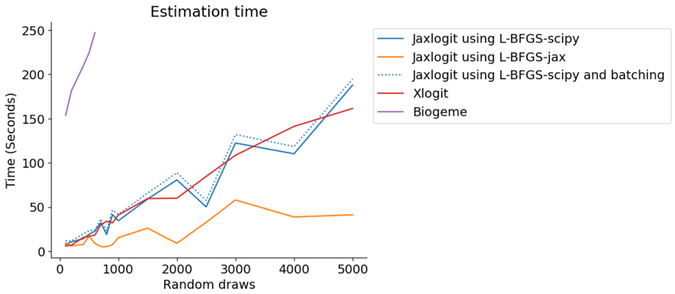
In the following chart, we show the estimated runtimes when applied to the electricity provider dataset. The first thing to note is that we were able to get Biogeme to estimate models, but its runtime quickly skyrocketed with the number of draws and eventually failed with out-of-memory errors when exceeding 600 draws. This is consistent with our expectations, given the general nature of the Biogeme solver and the relative performance characteristics previously reported by the xlogit authors.
When using the SciPy optimisation methods with BFGS and L-BFGS, jaxlogit performs similarly and slightly better than xlogit. We found that with the SciPy optimisation, it spent a lot of time copying the data between JAX and SciPy. Therefore, we achieved significant speed ups when using the JAX optimisation methods.
We aimed to make jaxlogit a meaningful extension of the existing ecosystem, driven by the requirements of estimating larger-than-usual problems. Through extensive testing and validation, we’ve demonstrated its reliability. The new features and performance gains from using JAX justify its creation. By simplifying input into jaxlogit, adapting examples from xlogit and adding our own, and implementing patterns from Scikit-Learn, we hope we’ve lowered the barrier to entry for discrete choice modellers familiar with the ecosystem.
As university students, it is exciting to think that as our code builds on others’ works from those specific to the scientific computing ecosystem, such as xlogit, JAX, SciPy, Pandas, etc to more general ecosystems like Sphinx for documentation and Jupytext Jupyter notebooks, others’ works can in the future build on our code.
There are a few promising extensions to jaxlogit that we didn’t have time to implement in the eight weeks of the internship. In mixed logit, the choice of random variable types could be expanded, and other models, such as probit and nested logit, could be added. Both of these additions would give more options to choice modellers.
One feature that xlogit supports is GPU acceleration. For jaxlogit, as the numerical calculations are handled by JAX, which supports GPU acceleration, there is a relatively unexplored avenue of performance improvements. We did some initial testing using an AMD GPU which worked quite seamlessly. Unfortunately, the initial results were a little inconclusive in terms of runtime improvement and we didn’t have sufficient time left to fully explore how these benefits could be fully realised.
Over the last two months, I have been interning with Outer Loop on the integration of web-based visualization …
Effective visualisation is critical for communicating the outputs of traffic forecasting models and studies, …
